

The Fourier Transform And Non-Periodic Waves
|
Now for the more general case. The Fourier Transform allows us to solve for non-periodic waves, while still allowing us to solve for periodic waves. It builds upon the Fourier Series. We now know that the Fourier Series rests upon the Superposition Principle, and the nature of periodic waves. The sinusoidal components are integer multiples of the fundamental frequency of a periodic wave. The fact that they are integer multiples allows us to use the orthogonality principle to extract the coefficients of the complex wave.
But, how do we apply this to non-periodic waves?
Note the following about periodic waves. The longer the wavelength of a periodic wave, the closer together the sinusoidal components will be along the frequency spectrum. In other words, the longer the fundamental wavelength, the smaller the fundamental frequency.
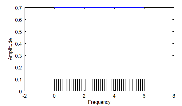
For example, we have three different fundamental wavelengths and their associated fundamental frequencies as shown below, equation 1:
Equation 1
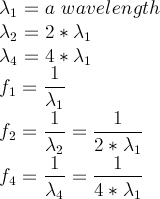
Now, if I were to plot the frequency domain for each of these fundamental frequencies I'd get the following three spectrum densities. The hash marks in the diagrams below represent the frequencies that are identifiable.
Above: diagram shows the density of frequencies you would see with fundamental frequency f1.
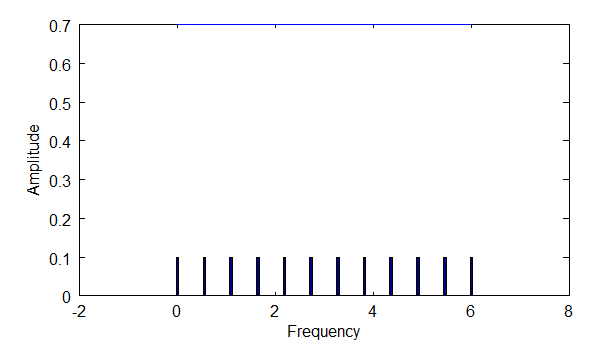
Above: diagram shows the density of frequencies you would see with f2, which is 2 times f1.
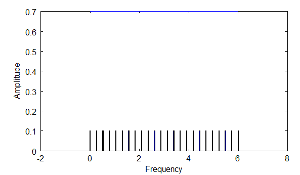
Above: diagram shows the density of frequencies you would see with f4, which is four times f1.
Notice that with longer wavelengths, you are able to find a higher density of frequencies via the orthogonality principle. Longer wavelengths mean smaller frequencies, and thus smaller steps between integer multiples.
So, then, extending the wavelength longer and longer will result in the density of frequencies identifiable along the spectrum increasing more and more. This means that as lambda --> infinity, f --> 0. F approaches zero, but never gets there.
Equation 2
At that point, all of the frequencies in the spectrum can be accounted for! This is what the Fourier Transform does. This allows you to deal with non-periodic waves.
However, the Fourier Transform no longer deals with integer multiples of the fundamental frequency. What happens is that you deal with all frequencies, and this affects the way you look at orthogonality, because between integer values there are non-zero areas. These non-zero areas are less than the values when the two sine waves are in sync, but they exist. These non-zero areas mean that this analysis is not ideal for finding sinusoids in a complex wave, but the method is still very good.
First, I'll give the equation for the Fourier Transform as it is usually given, with complex notation, equation 3.
Equation 3
That is nice compact notation, however in order to show better what is going on under the hood, I'll use sines and cosines. Here is a Fourier Transform in terms of sines and cosines, equation 4:
Equation 4
Notice the differences and similarities between the Fourier Coefficient equations for the Fourier Series and the Fourier Transform in equation 5, below.
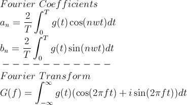
Equation 5
Some key differences. You don't divide by the period, T, or multiply by 2. Also, there are no longer integer multiples, i.e. 'n' is not in the Fourier Transform. You can select any frequency you want, which means you can also look at both periodic and non-periodic waves.
How the Fourier Transform Works
With Fourier Coefficients you find absolute values, since you are dividing by the period to get exact amplitudes for waves. However, with the Fourier Transform you only get the relative amplitude at different frequencies. This, however, is usually good enough.
Let's revisit the orthogonality principle. Remember, that the orthogonality principle gives a non-zero value when two sine waves have the same frequency, and a zero value when they have a different frequency, so long as we are dealing with integer multiples of the fundamental frequency. However, the Fourier Transform deals with all frequency values. So, here is how the orthogonality equation would look:
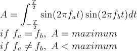
Equation 6
So, instead of zero, the values will be less than some maximum. The maximum is the peak value.
To show how the Fourier Transform works, I'll use this function, equation 7:
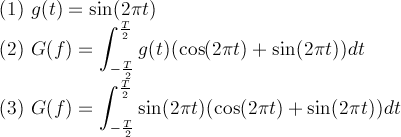
Equation 7
In equation 7, the simple wave (1) is plugged into (2) to get (3). Below are graphs showing the Fourier Transform plotted out as a spectrum. I've plotted it for three values of T in the diagrams below. The bigger the period, T, the higher the peak. So, as T approaches infinity, the peak becomes more and more pronounced. Also notice the "sidelobes". These are artifacts of the orthogonality principle when you are dealing with non-periodic waves, i.e. non-integer values of the fundamental frequency.
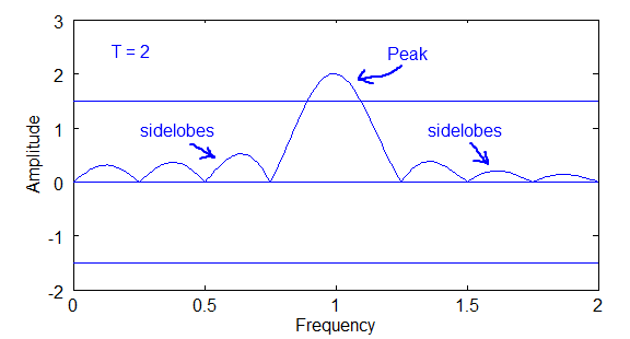
Above diagram of Fourier Transform plot for T=2
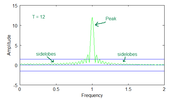
Above diagram of Fourier Transform plot for T=12
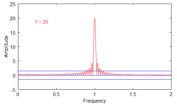
Above diagram of Fourier Transform plot for T=20
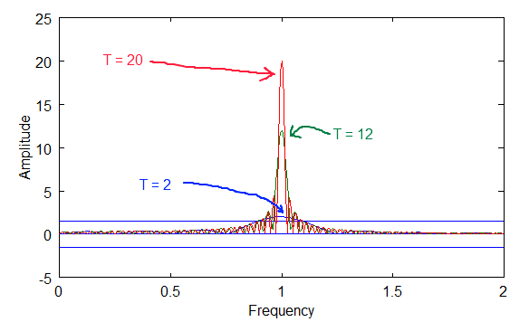
Above diagram of Fourier Transform plot for T=2, 12 and 20.
The last diagram above shows how the peaks overlap. Notice that the peaks get bigger with bigger periods, but the sidelobes stay in the same range.
Also, notice that the sinusoidal curve intersects zero at many points along the frequency axis for each of the T values. These zero intersections are the integer values for the fundamental, and the reason that the orthogonal principle is zero for the Fourier Series coefficients.
|